Most property managers using a pricing tool cannot answer a basic question: is it working? Bookings arrive, revenue fluctuates, and the assumption is that the model is contributing positively. That assumption is rarely tested. Without a structured evaluation framework, confidence in a pricing model is not evidence-based.
This article presents four methods for evaluating pricing model performance, ordered by analytical rigor. Each method is assessed for what it measures, where its validity breaks down, and which pricing model architectures are capable of supporting it.
One method commonly cited as a benchmark is excluded from this list. The reason for that exclusion is addressed at the end.
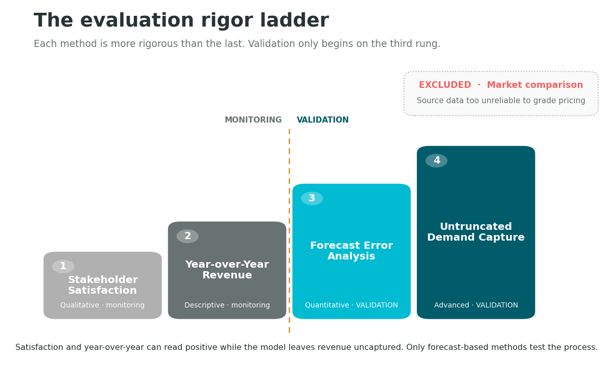
Method 1: Stakeholder Satisfaction
Analytical level: qualitative.
Owner and property manager satisfaction is the most widely used indicator of pricing performance. If revenue meets expectations, the model is assumed to be functioning. If an owner raises concerns, it is treated as a signal that something is wrong.
This indicator has legitimate value. Sustained satisfaction reflects consistent real-world performance. It captures contextual factors a model may take time to learn, including renovations, new market entrants, and operational changes. It also responds quickly to deteriorating performance, since dissatisfied owners escalate.
The core limitation is that satisfaction is unanchored. It measures perception relative to an unstated baseline, which may be prior-year revenue, pre-tool revenue, or an owner’s subjective sense of market conditions. Without a defined reference point, satisfaction is a qualitative signal, not a quantitative measurement.
This method functions as a monitoring indicator. It is not a performance validation.
When satisfaction is negative, it exposes a deeper problem: the absence of a scientific basis for explaining revenue outcomes. Dissatisfied owners ask specific questions. Why was the property vacant on a high-demand weekend? Why did rates decline when demand appeared strong? What decisions did the model make, and on what basis? These questions cannot be answered with owner satisfaction data alone. Answering them requires methods grounded in demand measurement, forecast accuracy, and documented pricing logic. Without those methods, property managers cannot explain outcomes with precision, only defend them with opinion.
Applicable to: all pricing model types.
Method 2: Year-Over-Year Revenue Comparison
Analytical level: descriptive.
Year-over-year revenue comparison is the most common quantitative benchmark in short-term rental performance evaluation. Current-period revenue is compared to the same period in the prior year. A positive variance is interpreted as evidence of model performance.
The method has practical strengths. It uses the same property as its own control, which eliminates cross-property variability. The data is consistently available. The comparison period shares seasonal structure with the current period.
However, the method has significant confounds that limit its validity as a measure of pricing model performance.
Market conditions are the primary confounder. Year-over-year revenue reflects demand trends, supply changes, platform algorithm shifts, and amenity improvements in addition to pricing decisions. A revenue increase in a rising market does not isolate the contribution of the pricing model. Conversely, a revenue decline in a softening market may reflect external conditions rather than model failure. To partially control for this, year-over-year comparisons should be paired with market-level RevPAR data for the same period.
Three additional factors introduce systematic bias:
Shifting holidays. Calendar position of holidays varies across years. A high-revenue holiday weekend falling within a comparison month in one year but not the other creates a revenue differential that has no relationship to pricing model behavior. Month-level comparisons are particularly susceptible to this distortion.
Owner usage. Changes in owner-blocked periods between comparison years alter available inventory. Revenue comparisons across periods with different night availability are not structurally equivalent. Valid comparisons should normalize to revenue per available night rather than total revenue.
Property maturity. New listings underperform their long-run revenue potential due to limited reviews, lower platform ranking, and insufficient historical data for pricing model calibration. A comparison against a property’s first year of operation will produce an artificially favorable variance in year two regardless of model performance. Portfolio-level analysis should apply same-store methodology, restricting comparisons to properties with stable operating histories in both periods.
Beyond these confounds, year-over-year comparison measures outcomes, not process. A property can show positive year-over-year revenue while the pricing model leaves substantial revenue uncaptured. The method confirms directional movement but cannot validate optimization.
A prerequisite constraint: this method is inapplicable to properties with less than one full year of operating history. Year-over-year comparison requires a prior-period baseline. For new listings, no such baseline exists.
Applicable to: all pricing model types, for properties with a minimum of one full year of operating history.
Method 3: Forecast Error Analysis
Analytical level: quantitative model validation.
Forecast error analysis is the first method that directly tests the internal validity of a pricing model. It compares a model’s forward revenue prediction against the actual observed outcome, producing a measurable error rate that can be tracked over time and used to assess model accuracy.
The process is as follows. At a defined point in the booking window, typically 60 days prior to a stay date, the model generates a revenue forecast for that date. After the date passes, the forecast is compared to actual revenue. The difference is the forecast error, expressed as a percentage of the forecast value.
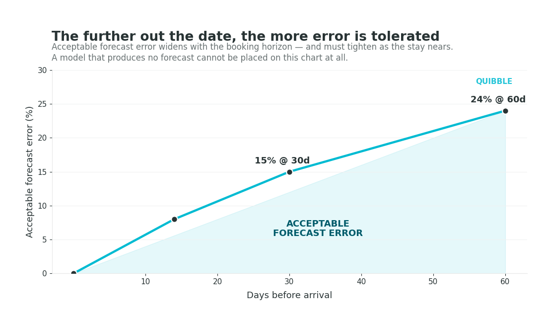
Revenue management literature establishes accepted error thresholds by booking horizon. At 60 days prior to arrival, forecast error below approximately 24% is considered acceptable. At 30 days, that threshold tightens to approximately 15%. In the final two weeks of the booking window, as the occupancy position clarifies, error should narrow further. Sustained forecast error outside these thresholds indicates model miscalibration.
The diagnostic value of this method is significant. A model that forecasts revenue accurately before a stay date has demonstrated empirically that it represents demand for that property. Forecast accuracy is evidence of model validity. A model with no forecasting capability has no comparable mechanism for self-validation. It generates prices without a forward revenue hypothesis and has no internal standard against which to measure its own accuracy.
Base price models cannot support this analysis. These models produce price adjustments relative to a calibration anchor. They do not generate forward revenue estimates. There is no forecast to compare against an observed outcome, and therefore no basis for forecast error analysis.
Applicable to: forecasting and optimization models only.
Method 4: Untruncated Demand Analysis
Analytical level: advanced quantitative validation.
Untruncated demand analysis extends beyond forecast accuracy to measure demand capture efficiency. It addresses a question forecast error analysis does not: did the model capture the demand that was available, or did pricing and restriction decisions cause bookable demand to go unobserved?
The central problem is demand truncation. Standard reservation data records observed transactions: a booking occurred at a given price on a given date. It does not record the demand that did not convert because the price exceeded the traveler’s willingness to pay, the minimum stay requirement excluded a viable booking, or the booking window was closed. This unobserved demand is structurally absent from the data a property manager can directly inspect.
Untruncated demand analysis uses statistical estimation methods to reconstruct total demand, including the portion that did not result in a booking. By comparing the demand the model captured against estimated total available demand, it is possible to compute a demand capture rate: the fraction of available revenue opportunity that the model converted to actual bookings.
A property that went vacant on a weekend with strong market demand did not fail due to absence of demand. It failed because the model priced above the demand curve for that market segment on that date. Untruncated demand analysis identifies that gap with precision.
This method requires that the model generate demand estimates. Without a forward demand signal, there is no reference point against which to measure capture. The analysis cannot be conducted on models that do not produce probabilistic demand forecasts.
Applicable to: optimization models with integrated demand forecasting only.
Excluded Method: Market Comparison
Excluded on data quality grounds.
The most commonly cited external benchmark is competitive set revenue comparison: measuring a property’s RevPAR against comparable listings in the same market to determine relative performance. This method is excluded from the framework because the underlying data does not support valid inference.
Competitive revenue data in the short-term rental industry is sourced primarily from scraped listing data, OTA partnership feeds, and operator surveys. Each of these sources carries substantial reliability limitations. Scraped data captures listed prices, not transaction prices, and occupancy must be inferred rather than observed directly. OTA partnership data is partial and subject to selection bias. Survey data depends on voluntary reporting and is subject to both response bias and measurement error. The aggregated figures published in market dashboards carry uncertainty that is not disclosed and cannot be quantified by the end user.
Competitive set definition introduces a second validity problem. Most market benchmarking tools define competitive sets geographically, using proximity as the primary criterion. A typical comp set may include hundreds or thousands of listings. The majority of these properties are not substitutes for any specific listing in the decision process of a prospective traveler. A benchmark constructed from an imprecise competitive set measures performance against an irrelevant reference group.
When source data is unreliable and the reference population is poorly defined, the resulting benchmark inherits both problems. Performance conclusions drawn from this method are not defensible with precision. Market comparison data may support broad directional assessments. It does not support rigorous attribution of pricing model performance.
Conclusion: Measurement Determines What Can Be Known
The validity of a pricing model evaluation is bounded by the method used to conduct it.
Stakeholder satisfaction and year-over-year comparison are monitoring indicators. They are operationally useful but insufficient for model validation. Both can produce positive readings while the pricing model leaves material revenue uncaptured. Neither method can identify the source of a performance shortfall with sufficient precision to support corrective action.
Forecast error analysis and untruncated demand capture are the validation standards applied in airline and hotel revenue management. These methods produce falsifiable hypotheses about model behavior and measure outcomes against defined quantitative thresholds. They are the appropriate standard for pricing model evaluation in short-term rental, and they are only accessible on models architecturally capable of generating demand forecasts.
A pricing model that does not produce forecasts cannot be rigorously evaluated. Operators using such models are measuring outcomes without the ability to assess the process that produced them. The evaluation gap is not a limitation of the operator. It is a limitation of the model.
Learn how Quibble’s forecasting engine lets you measure pricing performance, not just results.
Book a demo →
Related reading: Demand Forecasting for Short-Term Rentals · How Base Price Models Work · The End of the Base Price · Who Are Your Competitors